In the realm of digital images, every pixel seen on screens is fundamentally a mathematical construct — specifically a vector in a carefully defined color space. While the intuitive notion is to think of colors as singular entities, they are, in fact, points in a three-dimensional vector space where each dimension represents the intensity of a primary color. The most common representation, the RGB color space, encodes colors as triplets , where each component represents the intensity of red, green, and blue light respectively, typically scaled from 0 to 255 in 8-bit color depth.
But from the perspective of linear algebra, each color vector in this space can undergo various transformations, and these transformations are powered by the matrix multiplications and eigenvalues that define them. For any matrix acting on a vector , it is noticeable that the output is not arbitrary, but in reality scaled and rotated in ways determined by ‘s structure. When a transformation matrix has a dominant eigenvalue, , this eigenvalue shapes how the image data projects in that color space. Through these transformations, certain components or dimensions in the RGB color space may become reduced or highlighted, creating new perceptions of color by emphasizing or de-emphasizing specific wavelenghts. This effect is central to simulating color deficiencies like deuteranopia, where certain wavelenghts are perceived at a reduced intensity or even entirely omitted.
The mathematical beauty of this representation becomes apparent when we consider that any color transformation (brightness adjustment, saturation modification, or even simulation of color blindness) can be expressed as linear transformations. In linear algebra, this means applying a matrix multiplication to each color vector. For example, converting a color from RGB to grayscale isn’t simply averaging the three components, but a carefully weighted sum that accounts for human perception of different wavelengths. This transformation can be expressed as , these specific coefficients being derived from the human eye’s different sensitivities to red, green, and blue light.
Delving further into more complex color spaces, like YUV, as used in television transmission, we encounter transformations that separate luminance (Y) from chrominance (U and V). Represented as the matrix equation:
This demonstrates an essential principle of linear transformations: the ability to selectively emphasize or diminish certain dimensions in color space, allowing for compatibility with black-and-white broadcasting when color television was first introduced. The inverse transformation exists and remains linear, allowing the original RGB values to be reconstructed.
When simulating color blindness, linear transformations project the full color space onto a reduced subspace. In deuteranopia, for example, the transformation matrix alters the spectral sensitivities by effectively “removing” the green cone response, reducing the RGB space along this missing perceptual dimension. The transformation matrix is designed to project onto a two-dimensional plane within the RGB space, effectively simulating the loss of one color channel and highlighting the perceptual impacts on images.
Linear algebra further extends its utility in color manipulation through its ability to model more complex transformations. For example, a photographer adjusting the white balance is essentially applying a matrix transformation to shift the color vectors in response to different lightning conditions. This transformation matrix ensures the relationships between colors remain consistent while offsetting the overall color distribution.
Temperature and tint adjustments in photo editing can be viewed as specific rotations around an axis in the color space. When temperature is adjusted, the color vectors rotate around an axis orthogonal to both the blue-yellow and luminance axes, demonstrating another aspect of linear algebra’s power in manipulating vector spaces. The transformations’ additive and scalar properties mean multiple adjustments can be composed into a single transformation matrix, allowing cumulative effects to be captured efficiently through matrix multiplication.
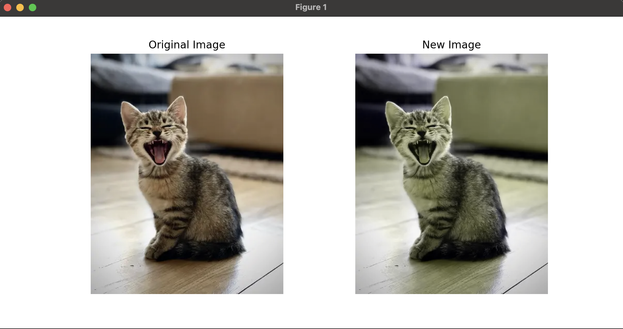
By utilizing a single matrix multiplication, the transformation of colors can respect both addition and scalar multiplication, while accurately projecting color onto a restricted subspace that mirrors the experience of individuals with deuteranopia, as seen in the following Python program. The algorithm implemented uses a transformation matrix derived from the research on color vision deficiencies and represents the projection of the full color space onto the reduced space available to individuals with this specific color blindness.
from PIL import Image
import numpy as np

def simulate_deuteranopia(image_path, output_path):
    # Load the image
    img = Image.open(image_path)
    img_array = np.array(img).astype(float)

    # Deuteranopia transformation matrix
    deuteranopia_matrix = np.array([
        [0.625, 0.375, 0],
        [0.7, 0.3, 0],
        [0, 0.3, 0.7]
    ])

    # Apply the transformation
    original_shape = img_array.shape
    pixels = img_array.reshape(-1, 3)
    transformed_pixels = np.dot(pixels, deuteranopia_matrix.T)
    transformed_pixels = np.clip(transformed_pixels, 0, 255)
    transformed_image = transformed_pixels.reshape(original_shape).astype(np.uint8)

    # Save and return the transformed image
    output_img = Image.fromarray(transformed_image)
    output_img.save(output_path)

    return output_img

def analyze_color_distribution(original_img, transformed_img):
    original_array = np.array(original_img)
    transformed_array = np.array(transformed_img)

    # Calculate average colors
    orig_avg = np.mean(original_array.reshape(-1, 3), axis=0)
    trans_avg = np.mean(transformed_array.reshape(-1, 3), axis=0)
    print("Original average RGB:", orig_avg)
    print("Transformed average RGB:", trans_avg)

    # Calculate color variance
    orig_var = np.var(original_array.reshape(-1, 3), axis=0)
    trans_var = np.var(transformed_array.reshape(-1, 3), axis=0)
    print("\nOriginal RGB variance:", orig_var)
    print("Transformed RGB variance:", trans_var)

import matplotlib.pyplot as plt

def compare_images(original_image, transformed_image):
    """Compare original and modified images side by side."""
    # Create a figure with two subplots
    fig, axs = plt.subplots(1, 2, figsize=(10, 5))

    # Display original image
    axs[0].imshow(original_image)
    axs[0].set_title("Original Image")
    axs[0].axis("off")

    # Display new image
    axs[1].imshow(transformed_image)
    axs[1].set_title("New Image")
    axs[1].axis("off")

    plt.show()

def main():
    input_path = "input_image.jpg"  # Replace with your image path
    output_path = "deuteranopia_simulation.jpg"

    # Apply transformation and analyze results
    original_img = Image.open(input_path)
    transformed_img = simulate_deuteranopia(input_path, output_path)
    analyze_color_distribution(original_img, transformed_img)

    # Compares both images
    compare_images(original_img, transformed_img)


if __name__ == "__main__":
    main()
The beauty of this approach lies in its elegance: a single matrix operation captures the complex physical and perceptual phenomena involved in color vision deficiency. The transformation preserves the mathematical properties expected — it’s linear, which means it respects the addition and scalar multiplication of colors, and it maps the color space in a way that accurately represents the perceptual experience of individuals with deuteranopia.